Implementing OLS

Now, let's proceed with the implementation of the Ordinary Least Squares (OLS) method. We'll begin by utilizing Python's built-in package to apply OLS. Following this, we will manually execute the OLS method, employing the formulas and expressions we derived in our earlier notes.

We will be using the GPA1 dataset from the text book "Introductory Econometrics, A Modern Approach 7e by Wooldridge" for our analysis.

Python regression

# importing libraries
import pandas as pd
import wooldridge
import numpy as np
import statsmodels.api as sm

# importing dataset
df = wooldridge.data('GPA1')

# Adding a constant (intercept) term to the independent variable
ind_var = sm.add_constant(df[['hsGPA','ACT']])

# Fit the OLS model
model = sm.OLS(df['colGPA'], ind_var).fit()

# Print the regression results
print(model.summary())

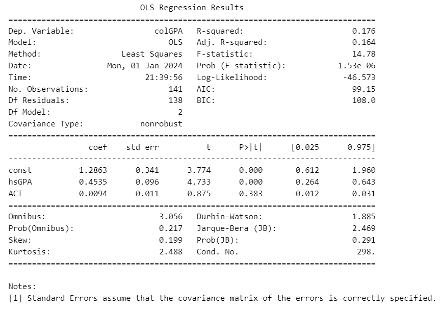
The econometric model is

$$\text{colGPA}_i= \beta_0 + \beta_1\text{hsGPA}_i + \beta_2\text{ACT}_i + \varepsilon_i.$$

The python regression gives us the following coefficients $(\bold{b})$ and standard errors $(\textbf{S.E})$

$$\begin{align*} \bold{b}= \begin{bmatrix} \hat{\beta}_0\\ \hat{\beta}_1\\ \hat{\beta}_2\\ \end{bmatrix}&= \begin{bmatrix} 1.29\\ 0.45\\ 0.009\\ \end{bmatrix},\\ \bold{S.E}&= \begin{bmatrix} 0.341\\ 0.096\\ 0.011\\ \end{bmatrix}.\\ \end{align*}$$

Manual regression

The dataset has $141$ observations, that is $n=141$. Consequently, the matrix $\bold{X}$ is of the dimension $141\times 3$, with the initial column being a constant column of ones, followed by 'hsGPA' and 'ACT' as the second and third column, respectively.

$\bold{y}$ is the 'colGPA' column.

Coefficients

$$\bold{b}=\bold{(X'X)}^{-1}\bold{X'y}.$$

# creating matrices
y=df['colGPA'].to_numpy()
X = sm.add_constant(df[['hsGPA','ACT']]).to_numpy()

# calculating b
b=(np.linalg.inv(X.T @ X))@ (X.T) @ y
b

array([1.28632777, 0.45345589, 0.00942601])

Standard Errors

We know that

$$\begin{align*} \mathbb{Var}(\bold{b|X})&=\frac{\bold{e'e}}{(n-K)}\bold{(X'X)}^{-1},\\ \bold{S.E}&=\sqrt{\mathbb{Var}(\bold{b|X})}=\sqrt{\frac{\bold{e'e}}{(n-K)}\bold{(X'X)}^{-1}}. \end{align*}$$

n,K=X.shape

# creating vector of residuals
e=y-X@b

# calculation S.E
se=(((e.T@e) * (np.linalg.inv(X.T @ X))) / (n-K))**(0.5)
se

array([[0.34082212, nan, nan],
[ nan, 0.09581292, nan],
[ nan, nan, 0.01077719]])

Reference

Example 3.1 "Introductory econometrics : a modern approach (Seventh). (2020). . Cengage Learning."