Estimation of Pi

GitHub repository

In this Jupyter notebook, we will estimate the value of $\boldsymbol{\pi}$.

Simulation

Procedure

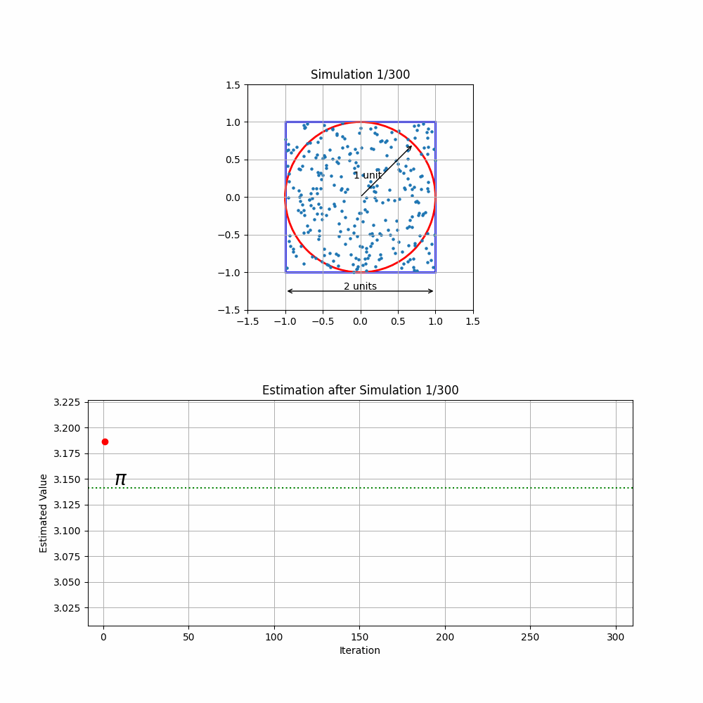
Consider a circle with a radius of 1 unit, perfectly fitting inside a square with 2-unit sides. If we randomly scatter 200 balls across the square, ensuring they're uniformly distributed, we can use the number of balls that land inside the circle to estimate the value of $\pi$.

Here's how it works:

The area of the circle is $\pi r^2$, and the area of the square is $(2r)^2$. Since the radius $r$ is 1 unit, the area of the circle is $\pi(1)² = \pi$, and the area of the square is $(2)^2$ = 4.

By calculating the ratio of the circle's area to the square's area and multiplying by 4, we get:

$$\frac{\text{Area of circle} \times 4}{\text{Area of square}} = \frac{\pi \times 1^2 \times 4}{2^2} = \pi$$

In our experiment, this ratio is represented by the number of balls that fall inside the circle relative to the total number of balls, multiplied by 4:

$$\frac{\text{Area of circle} \times 4}{\text{Area of square}} = \frac{\text{Number of balls in circle} \times 4}{\text{Total number of balls}}$$

Running this simulation 300 times (refer to the code below) and cumulatively calculating the ratio leverages the law of large numbers, leading to a more accurate estimation of $\pi$ as the number of trials increases. Each repetition refines our estimate, demonstrating how a simple physical model can mirror a complex mathematical principle.

Code for the Simulation

import matplotlib.pyplot as plt
import matplotlib.patches as patches
import numpy as np
import imageio
import os

n_iterations = 300
dots=300
np.random.seed(2609)
x, y = np.random.uniform(-1, 1, (n_iterations,dots)), np.random.uniform(-1, 1, (n_iterations,dots))
z=(x**2)+(y**2)
inside_square = np.full(n_iterations, dots)
inside_circle=np.sum(z <= 1,axis=1)
pi=(np.cumsum(inside_circle)/np.cumsum(inside_square))*4
filenames = []
div=np.arange(1,n_iterations+1)

for i in range(1, n_iterations + 1):
    fig, axs = plt.subplots(2, 1, figsize=(10, 10))

    fig.subplots_adjust(hspace=0.4)
    
    

    # Add a square patch
    square = patches.Rectangle((-1, -1), 2, 2, fill=False, color='blue', linewidth=2)
    axs[0].add_patch(square)

    # Add a circle patch
    circle = patches.Circle((0, 0), radius=1, fill=False, color='red', linewidth=2)
    axs[0].add_patch(circle)
    
    # Adding arrows
    axs[0].annotate('', xy=(-1,-1.25), xytext=(1, -1.25), arrowprops=dict(arrowstyle='<->', color='black'))
    axs[0].text(0, -1.23, '2 units', ha='center')

    axs[0].annotate('', xy=(0,0), xytext=( np.cos(np.pi/4),  np.sin(np.pi/4)), arrowprops=dict(arrowstyle='<-', color='black'))
    axs[0].text(0.1, 0.25, '1 unit', ha='center')

    # Set limits and aspect
    axs[0].set_xlim(-1.5, 1.5)
    axs[0].set_ylim(-1.5, 1.5)
    axs[0].set_aspect('equal', 'box')
    
    # Plots
    axs[0].scatter(x[i-1],y[i-1],s=5)
    axs[0].set_title(f'Simulation {i}/{n_iterations}')
    axs[0].grid()
    
    axs[1].plot(div[:i], pi[:i], color='blue')
    axs[1].plot(div[i-1], pi[i-1], color='r',marker='o')
    plt.xlim(min(div)-10, max(div)+10)
    plt.ylim(min(pi)-0.04, max(pi)+0.04)
    axs[1].set_title(f'Estimation after Simulation {i}/{n_iterations}')
    axs[1].set_xlabel("Iteration")
    axs[1].set_ylabel("Estimated Value")
    axs[1].axhline(y=np.pi, color='green', linestyle='dotted')
    axs[1].text(10, 3.144, '$\pi$', ha='center', fontsize=20)


    axs[1].grid()

    
    filename = f'frames/step_{i}.png'
    filenames.append(filename)
    plt.savefig(filename)
    plt.close()

# Create GIF
with imageio.get_writer('pi_est.gif', mode='I', duration=0.1) as writer:
    for filename in filenames:
        image = imageio.imread(filename)
        writer.append_data(image)

# Clean up the frames
for filename in filenames:
    os.remove(filename)