CART

Basics

Decision tree classification is a popular and intuitive machine learning technique used for both classification and regression tasks. The "Classification and Regression Tree" (CART) is a specific type of decision tree algorithm that focuses on binary decisions. The CART algorithm builds a tree structure where each internal node represents a decision based on a feature, each branch represents the outcome of that decision, and each leaf node represents a class label (in classification) or a value (in regression).

Algorithm

Objective of Growing a Regression Tree

• The goal of CART is to partition the data into distinct regions $R_1,R_2,…,R_M$ where the response variable (dependent variable) is modeled as a constant $c_m$​ in each region $R_m$.
• The function $f(x)$ represents the predicted value of the response for a given input $x$ and is defined as:

$$\begin{align*} f(x)=\sum_{m=1}^{M}c_m I(x \in R_m) \end{align*}$$

Here, $I(x \in R_m)$ is an indicator function that is 1 if $x$ belongs to region $R_m$ and 0 otherwise.

Choosing the Best Constants $\bold{c_m}$

• To determine the best $c_m$ for each region $R_m$, the criterion is to minimize the sum of squared errors between the observed values $y_i$ and the predicted value $f(x_i)$.
• The optimal $c_m$ is simply the average of the response variable $y_i$ within region $R_m$:

$$\begin{align*} \hat{c}_m=average(y_i|x_i\in R_m) \end{align*}$$

​ Finding the Optimal Binary Partition

• Finding the best binary partition (the best split) to minimize the sum of squared errors for the entire dataset is computationally challenging. Hence, CART uses a greedy algorithm to make this process feasible.
• The algorithm searches for the splitting variable $j$ and split point $s$ that divides the data into two regions:

$$\begin{align*} R_1​(j,s)=\{X∣X_j\leq ​s\}\text{ and }R_2​(j,s)=\{X∣X_j​ > s\} \end{align*}$$

• The objective is to find the pair $(j,s)$ that minimizes the sum of squared errors for the split:

$$\begin{align*} \min_{j,s}\bigg[\min_{c_1}\sum_{x_i\in R_1(j,s)}(y_i-c_1)^2 + \min_{c_2}\sum_{x_i\in R_2(j,s)}(y_i-c_2)^2\bigg] \end{align*}$$

• For each possible split $(j,s)$, the optimal constants $c_1$ and $c_2$ are computed as:

$$\begin{align*} \hat{c}_1=average(y_i|x_i\in R_1(j,s)) \text{ and }\hat{c}_2=average(y_i|x_i\in R_2(j,s)) \end{align*}$$

Greedy Search Process

• The algorithm evaluates all possible splits across all features to determine the best split. While this is still computationally demanding, it is feasible compared to evaluating all possible partitions of the data.
• Once the best split is found, the data is divided into two regions, and the process is repeated recursively for each resulting region, growing the tree.

Demonstration

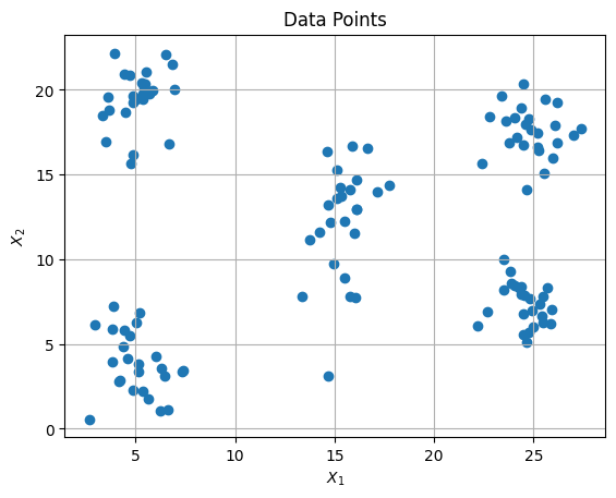
Here’s a demonstration of the CART Algorithm applied to the simulated data.

Data Generation

import matplotlib.pyplot as plt
import pandas as pd
import numpy as np
from sklearn.tree import DecisionTreeClassifier
from sklearn.tree import plot_tree


np.random.seed(2609)
x1=np.random.normal(loc=5,scale=1,size=25)
x2=np.random.normal(loc=5,scale=2,size=25)
data1=pd.DataFrame({'X_1':x1,'X_2':x2,'y_1':'R1','y_2':2})

x1=np.random.normal(loc=5,scale=1,size=25)
x2=np.random.normal(loc=20,scale=2,size=25)
data2=pd.DataFrame({'X_1':x1,'X_2':x2,'y_1':'R2','y_2':0})

x1=np.random.normal(loc=15,scale=1,size=25)
x2=np.random.normal(loc=12.5,scale=3,size=25)
data3=pd.DataFrame({'X_1':x1,'X_2':x2,'y_1':'R3','y_2':5})

x1=np.random.normal(loc=25,scale=1,size=25)
x2=np.random.normal(loc=7.5,scale=1.5,size=25)
data4=pd.DataFrame({'X_1':x1,'X_2':x2,'y_1':'R4','y_2':6})

x1=np.random.normal(loc=25,scale=1,size=25)
x2=np.random.normal(loc=17.5,scale=1.5,size=25)
data5=pd.DataFrame({'X_1':x1,'X_2':x2,'y_1':'R5','y_2':7})

data=pd.concat([data1,data2,data3,data4,data5],axis=0).reset_index(drop=True)

plt.scatter(data['X_1'],data['X_2'])
plt.xlabel(r'$X_1$')
plt.ylabel(r'$X_2$')
plt.title('Data Points')
plt.grid(axis='y')
plt.show()

Model Fitting

cart_tree = DecisionTreeClassifier()
cart_tree.fit(data[['X_1','X_2']], data['y_2'])

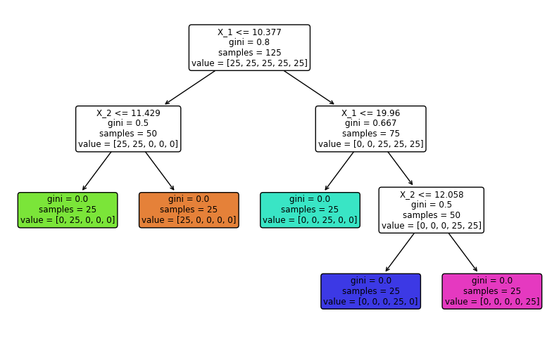
Tree Representation

# Plot the decision tree
plt.figure(figsize=(10, 6))  
plot_tree(cart_tree, filled=True, feature_names=['X_1', 'X_2'], rounded=True)
plt.show()

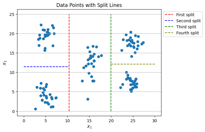
Plotting Data Points with Split Lines

tree = cart_tree.tree_
# Access the feature indices and threshold values
feature = tree.feature
threshold = tree.threshold

# Create a list to store split points
split_points = []

# Iterate over all nodes in the tree
for i in range(tree.node_count):
    if feature[i] != -2:  # -2 indicates a leaf node
        split_points.append((feature[i], threshold[i]))

X_1_splitting_points=[s[1] for s in split_points if s[0]==0]
X_2_splitting_points=[s[1] for s in split_points if s[0]==1]

# Plotting
plt.scatter(data['X_1'],data['X_2'])

plt.vlines(X_1_splitting_points[0], ymin=0, ymax=25, colors='r', linestyles='dashed',label='First split')

plt.hlines(X_2_splitting_points[0], xmin=0, xmax=X_1_splitting_points[0], colors='b', linestyles='dashed',label='Second split')

plt.vlines(X_1_splitting_points[1], ymin=0, ymax=25, colors='g', linestyles='dashed',label='Third split')

plt.hlines(X_2_splitting_points[1], xmin=X_1_splitting_points[1], xmax=30, colors='olive', linestyles='dashed',label='Fourth split')
     
plt.xlabel(r'$X_1$')
plt.ylabel(r'$X_2$')
plt.title('Data Points with Split Lines')
plt.grid(axis='y')
plt.legend(loc='upper left', bbox_to_anchor=(1, 1))
plt.show()

References

1. Hastie, T. "The Elements of Statistical Learning: Data Mining, Inference, and Prediction." (2009).